Tropical Moist Forests

Tropical moist forest (TMF) climatic niche distributions were projected at the end of the century (2070-2100) using downscaled CMIP6 and CORDEX projections for scenario 2.6 and 8.5. Specifically, we used the definition from Holdridge 1967 (Holdridge and Tosi Jr 1967) as areas with a mean annual temperature over 16°C, a total annual precipitation over 1,000 \(mm~yr^{-1}\), and a ratio of potential evapotranspiration over precipitation below 1. Potential evaportanspiration (pet, \(mm~month^{-1}\)) was derived from monthly mean, maximum and minimum temperatures (tas, tasmax, tasmin, °C) and surface downward short-wave radiation (rsds, \(MJ~m^{-~2}~month^{-1}\)) as:

\[ pet = 0.0023 \times rsds \times (tas + 17.8) \times (tasmax - tasmin)^{0.5} \]

Surface downward short-wave radiation was derived from CHELSA 2 historical climatologies and assumed constant.

Current

Code

files <- list.files("outputs/tmf_hist", full.names = TRUE)
names(files) <- c("Côte-d'Ivoire", "French-Guiana", "New-Caledonia")
tmf <- files %>%
  lapply(rast) %>%
  lapply(as.data.frame, xy = TRUE) %>%
  bind_rows(.id = "area") %>%
  mutate(y = ifelse(area == "New-Caledonia", -y, y)) %>%
  na.omit()
write_tsv(tmf, "outputs/current_tmf.tsv")

Code

g <- read_tsv("outputs/current_tmf.tsv") %>%
  mutate(area = ifelse(area == "Côte-d'Ivoire", "Ivory-Coast", area)) %>%
  mutate(area = gsub("-", " ", area)) %>%
  ggplot(aes(x, y, fill = as.character(tmf))) +
  geom_raster() +
  facet_wrap(~area, scales = "free") +
  theme_bw() +
  scale_fill_manual(guide = "none", values = c("darkgrey", "#48712d")) +
  theme(
    axis.title = element_blank(),
    axis.ticks = element_blank(),
    axis.text = element_blank(),
    panel.border = element_blank(),
    panel.grid = element_blank(),
    panel.background = element_rect(fill = "white"),
    panel.spacing = unit(0, "lines"),
    aspect.ratio = 1
  )
ggsave("figures/fs07.png", g, dpi = 800, bg = "white", width = 8)
g

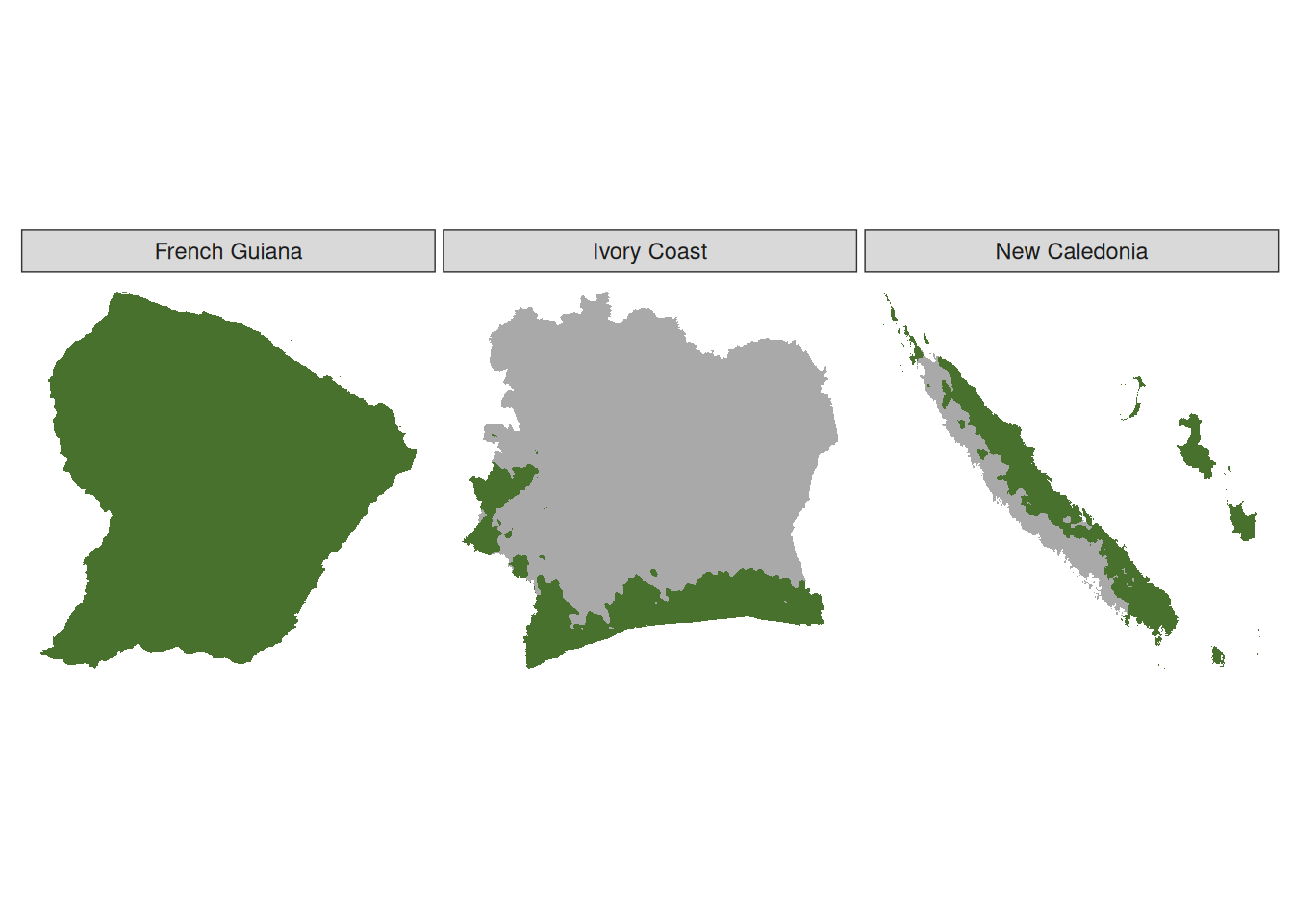
Fig. S7. Current distribution of the climate niche of the tropical moist forests in Ivory Coast, French Guiana and New Caledonia. The climate niche has been defined based on CHELSA2 data for the 1980-2005 period using Holdridge (1967)’s definition of areas with a mean annual temperature over 16°C, a total annual precipitation over 1,000 mm, and a ratio of potential evapotranspiration over precipitation below 1. Potential evapotranspiration (pet) was derived from monthly mean, maximum and minimum temperatures (tas, tasmax, tasmin) and surface downward short-wave radiation (rsds) as pet = 0.0023 x rsds x (tas+17.8) x (tasmax - tasmin)^0.5.

Projected

Code

index <- data.frame(
  file = list.files("results/tmf/nc/", full.names = FALSE),
  path = list.files("results/tmf/nc/", full.names = TRUE)
) %>%
  separate(file, c(
    "country", "project", "domain", "institute", "model", "experiment",
    "ensemble", "rcm", "downscaling", "base", "aggregation",
    "period_future", "period_present", "period_hist"
  ), sep = "_", remove = FALSE)
files <- index %>%
  select(country, project, experiment) %>%
  unique()
for (r in seq_len(nrow(files))) {
  filter(
    index,
    country == files$country[r],
    project == files$project[r],
    experiment == files$experiment[r]
  )$path %>%
    lapply(rast, lyrs = "tmf") %>%
    rast() %>%
    sum() %>%
    writeRaster(
      filename = paste0(
        "outputs/tmf/",
        files$country[r], "_",
        files$project[r], "_",
        files$experiment[r], ".tif"
      ),
      overwrite = TRUE
    )
}

Code

fg <- rast(c(
  list.files("outputs/tmf/", pattern = "Guiana", full.names = TRUE),
  "outputs/tmf_hist/French-Guiana.nc"
))
names(fg) <- c("CMIP6_2.6", "CMIP6_8.5", "CORDEX_2.6", "CORDEX_8.5", "hist")
fg_tab <- as.data.frame(fg, xy = TRUE, na.rm = FALE) %>%
  mutate_at(
    c("CMIP6_2.6", "CMIP6_8.5", "CORDEX_2.6", "CORDEX_8.5"),
    ~ . / max(abs(.), na.rm = TRUE)
  ) %>%
  gather(projection, tmf, -x, -y, -hist) %>%
  separate(projection, c("project", "experiment"), "_") %>%
  mutate(project = factor(project, levels = c("CMIP6", "CORDEX"))) %>%
  na.omit() %>%
  mutate(agreement = abs(tmf) * 100) %>%
  mutate(type = ifelse(tmf >= 0, "gain", "loss")) %>%
  mutate(type = ifelse(tmf == 0, "stable", type)) %>%
  mutate(type = ifelse(hist == 0 & tmf == 0, "non-forest", type)) %>%
  mutate(agreement = ifelse(type %in% c("stable", "non-forest"),
    100, agreement
  ))
write_tsv(fg_tab, "outputs/fg_tmf.tsv")
ci <- rast(c(
  list.files("outputs/tmf/", pattern = "Ivoire", full.names = TRUE),
  "outputs/tmf_hist/Côte-d'Ivoire.nc"
))
names(ci) <- c("CMIP6_2.6", "CMIP6_8.5", "CORDEX_2.6", "CORDEX_8.5", "hist")
ci_tab <- as.data.frame(ci, xy = TRUE, na.rm = FALSE) %>%
  mutate_at(
    c("CMIP6_2.6", "CMIP6_8.5", "CORDEX_2.6", "CORDEX_8.5"),
    ~ . / max(abs(.), na.rm = TRUE)
  ) %>%
  gather(projection, tmf, -x, -y, -hist) %>%
  separate(projection, c("project", "experiment"), "_") %>%
  mutate(project = factor(project, levels = c("CMIP6", "CORDEX"))) %>%
  na.omit() %>%
  mutate(agreement = abs(tmf) * 100) %>%
  mutate(type = ifelse(tmf >= 0, "gain", "loss")) %>%
  mutate(type = ifelse(tmf == 0, "stable", type)) %>%
  mutate(type = ifelse(hist == 0 & tmf == 0, "non-forest", type)) %>%
  mutate(agreement = ifelse(type %in% c("stable", "non-forest"),
    100, agreement
  ))
write_tsv(ci_tab, "outputs/ci_tmf.tsv")
nc <- rast(c(
  list.files("outputs/tmf/", pattern = "Caledonia", full.names = TRUE),
  "outputs/tmf_hist/New-Caledonia.nc"
))
names(nc) <- c("CMIP6_2.6", "CMIP6_8.5", "CORDEX_2.6", "CORDEX_8.5", "hist")
nc_tab <- as.data.frame(nc, xy = TRUE, na.rm = FALSE) %>%
  mutate_at(
    c("CMIP6_2.6", "CMIP6_8.5", "CORDEX_2.6", "CORDEX_8.5"),
    ~ . / max(abs(.), na.rm = TRUE)
  ) %>%
  gather(projection, tmf, -x, -y, -hist) %>%
  separate(projection, c("project", "experiment"), "_") %>%
  mutate(project = factor(project, levels = c("CMIP6", "CORDEX"))) %>%
  na.omit() %>%
  mutate(y = -y) %>%
  mutate(agreement = abs(tmf) * 100) %>%
  mutate(type = ifelse(tmf >= 0, "gain", "loss")) %>%
  mutate(type = ifelse(tmf == 0, "stable", type)) %>%
  mutate(type = ifelse(hist == 0 & tmf == 0, "non-forest", type)) %>%
  mutate(agreement = ifelse(type %in% c("stable", "non-forest"),
    100, agreement
  ))
write_tsv(nc_tab, "outputs/nc_tmf.tsv")

Code

g <- vroom("outputs/fg_tmf.tsv") %>%
  mutate(experiment = paste0(experiment, "~W~m^{-~2}")) %>%
  mutate(type = recode(type,
    "stable" = "stable forest",
    "non-forest" = "stable non-forest"
  )) %>%
  ggplot(aes(x, y, fill = type, alpha = agreement)) +
  geom_raster() +
  coord_equal() +
  facet_grid(experiment ~ project, labeller = label_parsed) +
  theme_bw() +
  theme(
    axis.title = element_blank(),
    axis.ticks = element_blank(),
    axis.text = element_blank(),
    panel.border = element_blank(), panel.grid = element_blank(),
    panel.background = element_rect(fill = "white")
  ) +
  scale_fill_manual("Forest cover change:",
    values = c("#e40400", "black")
  ) +
  scale_alpha_continuous("Model Agreement for gain and loss (%)",
                         range = c(.1, 1)) +
  theme(legend.position = "bottom", legend.box = "vertical")
ggsave("figures/fs08.png", g, dpi = 800, bg = "white", width = 8)
g

Fig. S8. Tropical moist forest ditribution predicted in French Guiana by the end of the century for CMIP6 and CORDEX model with scenario 2.6 and 8.5.

Code

g <- vroom("outputs/ci_tmf.tsv") %>%
  mutate(experiment = paste0(experiment, "~W~m^{-~2}")) %>%
  mutate(type = recode(type,
    "stable" = "stable forest",
    "non-forest" = "stable non-forest"
  )) %>%
  ggplot(aes(x, y, fill = type, alpha = agreement)) +
  geom_raster() +
  coord_equal() +
  facet_grid(experiment ~ project, labeller = label_parsed) +
  theme_bw() +
  theme(
    axis.title = element_blank(),
    axis.ticks = element_blank(),
    axis.text = element_blank(),
    panel.border = element_blank(), panel.grid = element_blank(),
    panel.background = element_rect(fill = "white")
  ) +
  scale_fill_manual("Forest cover change:",
    values = c("#48712d", "#e40400", "black", "darkgrey")
  ) +
  scale_alpha_continuous("Model Agreement for gain and loss (%)",
                         range = c(.1, 1)) +
  theme(legend.position = "bottom", legend.box = "vertical")
ggsave("figures/fs09.png", g, dpi = 800, bg = "white", width = 8)
g

Fig. S9. Tropical moist forest ditribution predicted in Ivory Coast by the end of the century for CMIP6 and CORDEX model with scenario 2.6 and 8.5.

Code

g <- vroom("outputs/nc_tmf.tsv") %>%
  mutate(experiment = paste0(experiment, "~W~m^{-~2}")) %>%
  mutate(type = recode(type,
    "stable" = "stable forest",
    "non-forest" = "stable non-forest"
  )) %>%
  ggplot(aes(x, y, fill = type, alpha = agreement)) +
  geom_raster() +
  coord_equal() +
  facet_grid(experiment ~ project, labeller = label_parsed) +
  theme_bw() +
  theme(
    axis.title = element_blank(),
    axis.ticks = element_blank(),
    axis.text = element_blank(),
    panel.border = element_blank(), panel.grid = element_blank(),
    panel.background = element_rect(fill = "white")
  ) +
  scale_fill_manual("Forest cover change:",
    values = c("#48712d", "#e40400", "black", "darkgrey")
  ) +
  scale_alpha_continuous("Model Agreement for gain and loss (%)",
                         range = c(.1, 1)) +
  theme(legend.position = "bottom", legend.box = "vertical")
ggsave("figures/fs10.png", g, dpi = 800, bg = "white", width = 8)
g

Fig. S10. Tropical moist forest ditribution predicted in New Caledonia by the end of the century for CMIP6 and CORDEX model with scenario 2.6 and 8.5.

Code

tmf <- list(
  "French Guiana" = "outputs/fg_tmf.tsv",
  "Ivory Coast" = "outputs/ci_tmf.tsv",
  "New Caledonia" = "outputs/nc_tmf.tsv"
) %>%
  lapply(vroom) %>%
  bind_rows(.id = "country") %>%
  filter(experiment == "2.6")
g <- tmf %>%
  mutate(country = factor(country,
    levels = c(
      "French Guiana",
      "Ivory Coast",
      "New Caledonia"
    )
  )) %>%
  mutate(type = recode(type,
    "stable" = "stable forest",
    "non-forest" = "stable non-forest"
  )) %>%
  mutate(project_country = paste(project, country)) %>%
  ggplot(aes(x, y, fill = type, alpha = agreement)) +
  geom_raster() +
  facet_wrap(~project_country, scales = "free") +
  theme_bw() +
  theme(
    axis.title = element_blank(),
    axis.ticks = element_blank(),
    axis.text = element_blank(),
    panel.border = element_blank(), panel.grid = element_blank(),
    panel.background = element_rect(fill = "white")
  ) +
  scale_fill_manual("Forest cover change:",
    values = c("#48712d", "#e40400", "black", "darkgrey")
  ) +
  scale_alpha_continuous("Model Agreement for gain and loss (%)",
                         range = c(.1, 1)) +
  theme(legend.position = "bottom", legend.box = "vertical")
ggsave("figures/f04.png", g, dpi = 300, width = 8, height = 7, bg = "white")
g

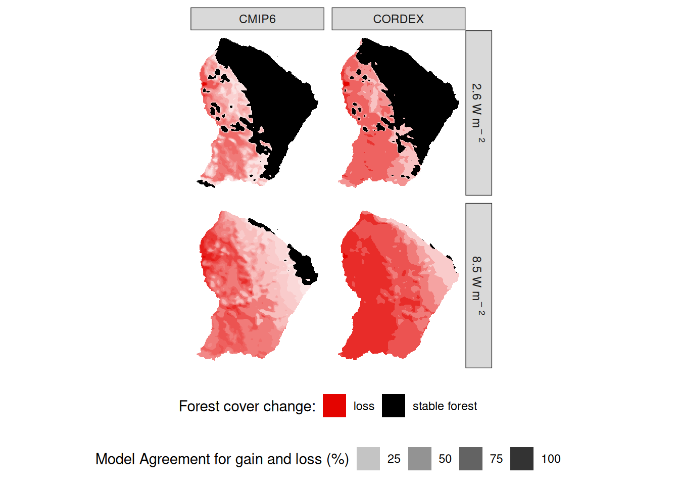
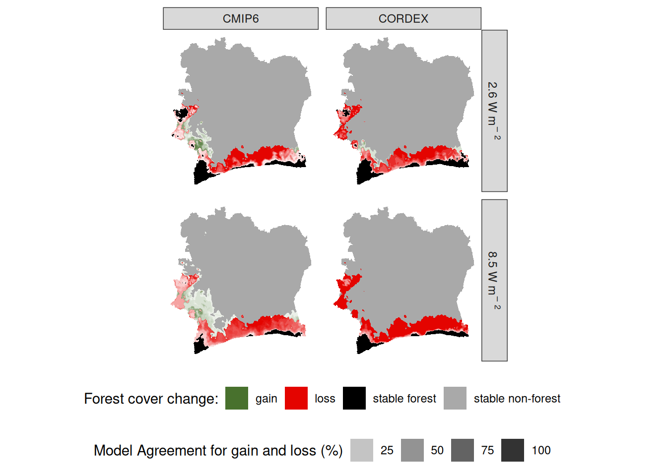
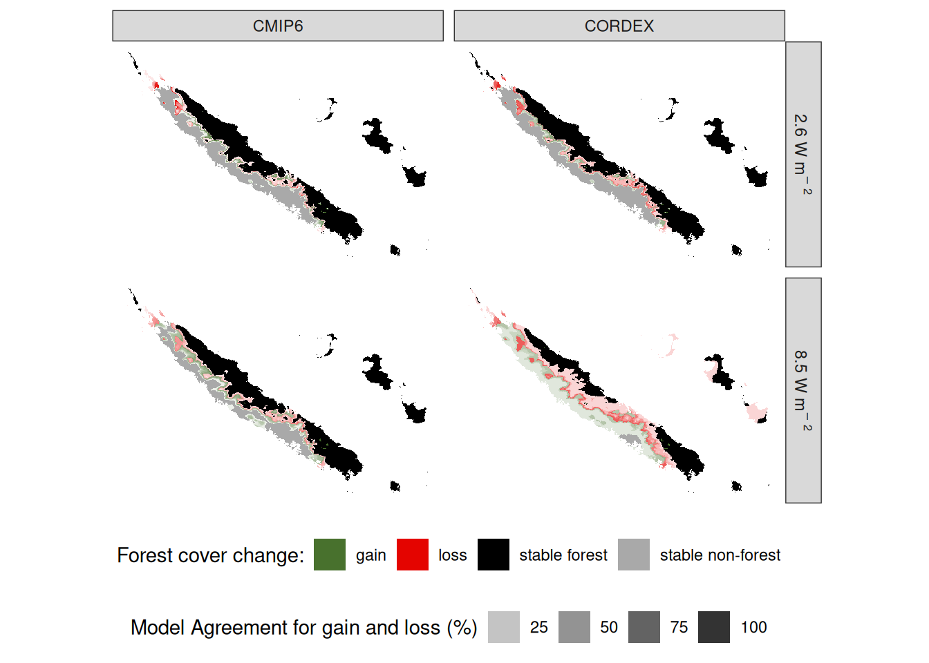
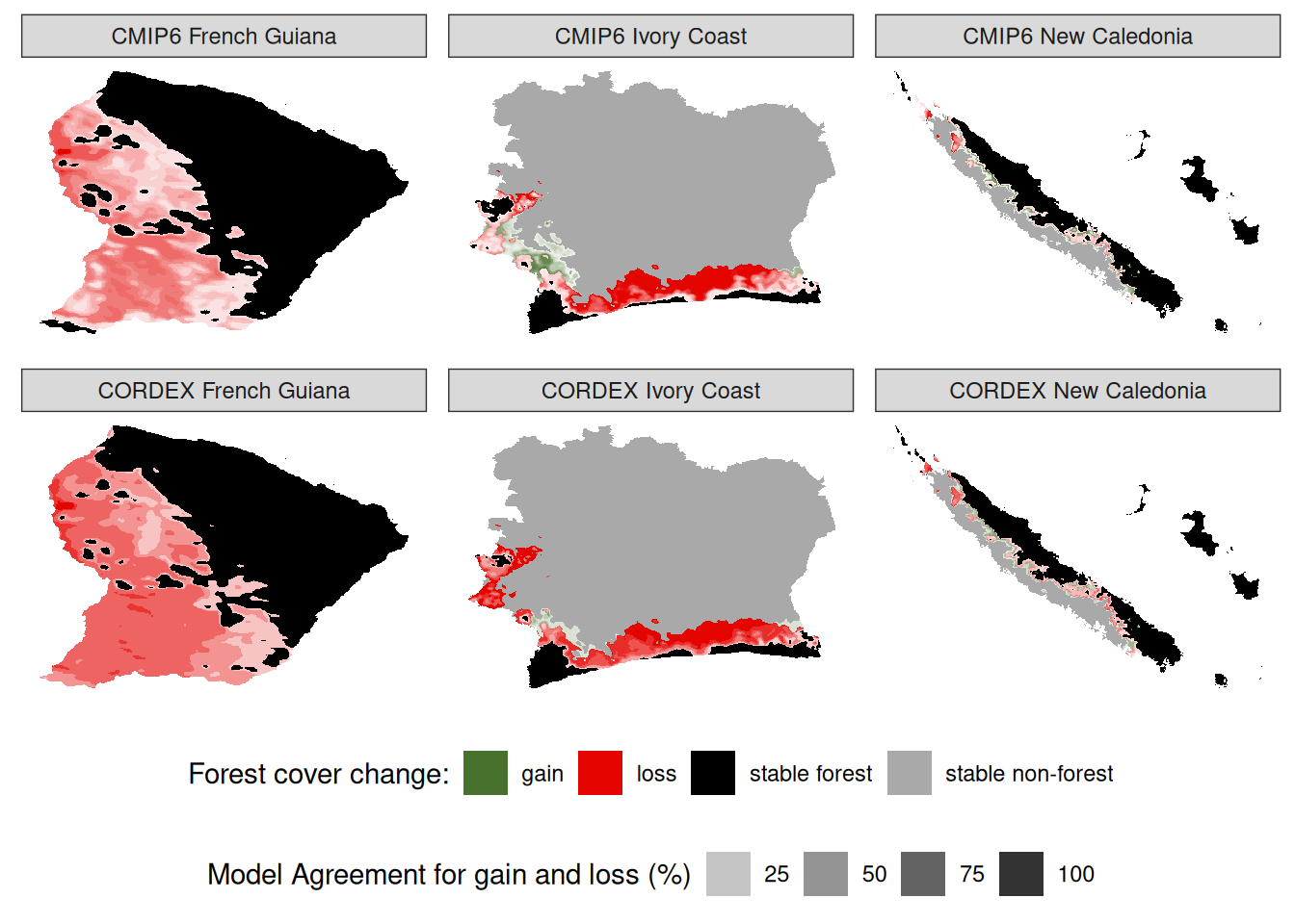
Fig. 4. Projected climate niche shift of the tropical moist forest by the end of the century. The tropical moist forest climatic niche has been projected for the period 2070-2100 based on downscaled projections from CORDEX and CMIP6 for mean, minimum and maximum monthly temperature and monthly precipitation. The projected climatic niches were compared with the current climatic niche for each model and scenario to calculate shifts with loss (red) or gain (green) of forest. The maps show with colour intensity in Ivory Coast, French Guiana and New Caledonia the agreement between models in shifts for scenario 2.6 with CMIP6 and CORDEX projections. Black pixels indicate areas of stable forest, while grey pixels indicate areas of historical and projection stable non-forest. Current distribution of the climate niche of the tropical moist forests can be found in Supplementary Figure S7, while details on Ivory Coast, French Guiana and New Caledonia for both CORDEX and CMIP6 and scenarios 2.6 and 8.5 can be found in Supplementary Figures S8, S9, and S10.Means across CMIP6 and CORDEX projections for both scenario 2.6 and 8.5 are shown in Fig. S11.

Code

tmf <- list(
  "French Guiana" = "outputs/fg_tmf.tsv",
  "Ivory Coast" = "outputs/ci_tmf.tsv",
  "New Caledonia" = "outputs/nc_tmf.tsv"
) %>%
  lapply(vroom) %>%
  bind_rows(.id = "country") %>%
  select(country, x, y, hist, experiment, project, tmf) %>%
  pivot_wider(names_from = project, values_from = tmf) %>%
  rowwise() %>%
  mutate(tmf = mean(c(CMIP6, CORDEX))) %>%
  ungroup() %>%
  select(-CMIP6, -CORDEX) %>%
  mutate(agreement = abs(tmf) * 100) %>%
  mutate(type = ifelse(tmf >= 0, "gain", "loss")) %>%
  mutate(type = ifelse(tmf == 0, "stable", type)) %>%
  mutate(type = ifelse(hist == 0 & tmf == 0, "non-forest", type)) %>%
  mutate(agreement = ifelse(type %in% c("stable", "non-forest"),
    100, agreement
  ))
g <- tmf %>%
  mutate(type = recode(type,
    "stable" = "stable forest",
    "non-forest" = "stable non-forest"
  )) %>%
  mutate(experiment = recode(as.character(experiment),
    "2.6" = "~2.6~W~m^{-~2}",
    "8.5" = "~8.5~W~m^{-~2}"
  )) %>%
  mutate(country = gsub(" ", "~", country)) %>%
  mutate(experiment_country = paste0(country, experiment)) %>%
  mutate(experiment_country = factor(experiment_country,
    levels = c(
      "French~Guiana~2.6~W~m^{-~2}",
      "Ivory~Coast~2.6~W~m^{-~2}",
      "New~Caledonia~2.6~W~m^{-~2}",
      "French~Guiana~8.5~W~m^{-~2}",
      "Ivory~Coast~8.5~W~m^{-~2}",
      "New~Caledonia~8.5~W~m^{-~2}"
    )
  )) %>%
  ggplot(aes(x, y, fill = type, alpha = agreement)) +
  geom_raster() +
  facet_wrap(~experiment_country, scales = "free", labeller = label_parsed) +
  theme_bw() +
  theme(
    axis.title = element_blank(),
    axis.ticks = element_blank(),
    axis.text = element_blank(),
    panel.border = element_blank(), panel.grid = element_blank(),
    panel.background = element_rect(fill = "white")
  ) +
  scale_fill_manual("Forest cover change:",
    values = c("#48712d", "#e40400", "black", "darkgrey")
  ) +
  scale_alpha_continuous("Model Agreement for gain and loss (%)",
                         range = c(.1, 1)) +
  theme(legend.position = "bottom", legend.box = "vertical")
ggsave("figures/fs11.png", g, dpi = 800, bg = "white", width = 8)
g

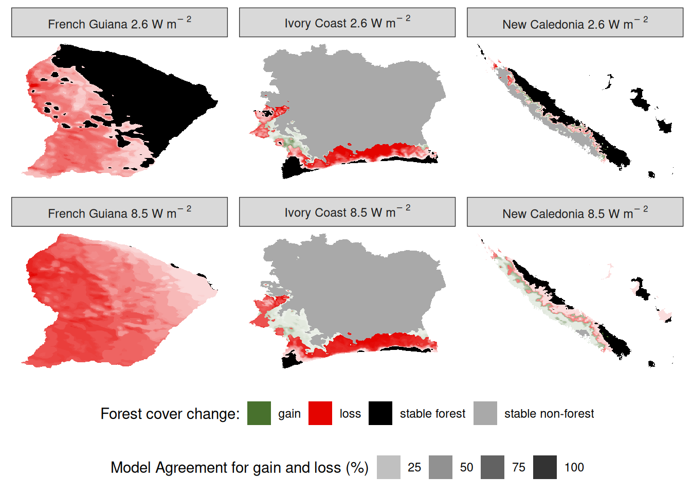
Fig. S11. Projected climate niche shift of the tropical moist forest by the end of the century. The tropical moist forest climatic niche has been projected for the period 2070-2100 based on downscaled projections from CORDEX and CMIP6 for mean, minimum and maximum monthly temperature and monthly precipitation. The projected climatic niches were compared with the current climatic niche for each model and scenario to calculate shifts with loss (red) or gain (green) of forest. The maps show with colour intensity in Ivory Coast, French Guiana and New Caledonia the agreement between models in shifts for scenarios 2.6 and 8.5 with the means across CMIP6 and CORDEX projections. Black pixels indicate areas of stable forest, while grey pixels indicate areas of historical and projection stable non-forest.

Holdridge, LR, and Joseph A Tosi Jr. 1967. “Tropical Science Center: San Jose, Costa Rica.” Life Zone Ecology; Tropical Science Center: San Jose, Costa Rica.