MeteoFrance

Code

weather <- list.files("data", pattern = "gz", full.names = TRUE) %>%
  read_delim(locale = locale(decimal_mark = "."), delim = ";") %>%
  select(NOM_USUEL, LAT, LON, AAAAMM, RR, TM, TMMAX, TMMIN) %>%
  rename_all(tolower) %>%
  rename(loc = nom_usuel, pr = rr, tas = tm, tasmin = tmmin, tasmax = tmmax) %>%
  mutate(pr = as.numeric(pr)) %>%
  mutate(aaaamm = as.character(aaaamm)) %>%
  mutate(year = str_sub(aaaamm, 1, 4), month = str_sub(aaaamm, 5, 6)) %>%
  mutate(date = as_date(paste0(year, "-", month, "-01"))) %>%
  select(loc, lat, lon, date, pr, tas, tasmin, tasmax)
climate <- weather %>%
  filter(year(date) %in% 2006:2019) %>%
  group_by(loc, year(date)) %>%
  filter(n() == 12) %>%
  group_by(loc) %>%
  mutate(n_year = n() / 12) %>%
  filter(n_year >= 6) %>%
  group_by(loc, lat, lon, n_year, month = month(date)) %>%
  summarise_all(mean, na.omit = TRUE) %>%
  mutate(country = ifelse(lon > 0, "New Caledonia", "French Guiana"))
xy <- climate %>%
  select(loc, lat, lon) %>%
  unique() %>%
  st_as_sf(coords = c("lon", "lat"), crs = 4326)

Code

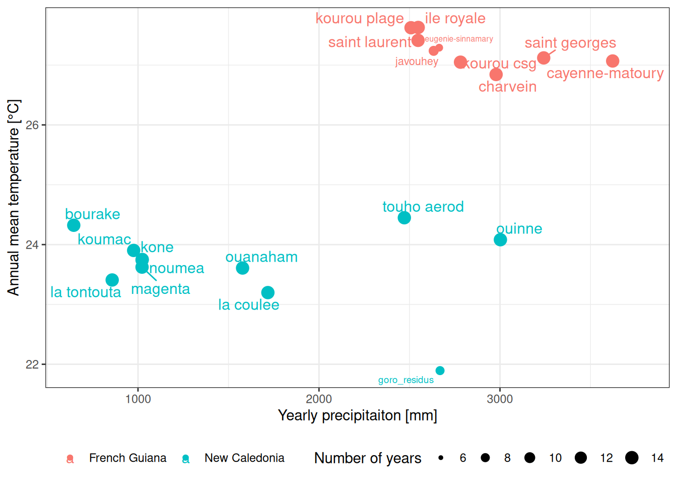
g <- climate %>%
  group_by(country, loc, n_year, lat, lon) %>%
  summarise(pr = sum(pr), tas = mean(tas)) %>%
  ggplot(aes(pr, tas, label = tolower(loc), col = country, size = n_year)) +
  geom_point() +
  ggrepel::geom_text_repel() +
  theme_bw() +
  xlab("Yearly precipitaiton [mm]") +
  ylab("Annual mean temperature [°C]") +
  theme(legend.position = "bottom") +
  scale_size_continuous("Number of years", range = c(1, 4)) +
  scale_color_discrete("")
ggsave("figures/fs05.png", g, dpi = 800, bg = "white", width = 8)
g

Fig S5. Yearly precipitation and mean temperature from punctual Meteo-France data for the period 2006-2019 with a minimum of 6 complete years in French Guiana (red) and New Caledonia (blue). Point size represents the number of complete years in the data.

Code

clim <- climate %>%
  ungroup() %>%
  select(-lat, -lon, -date, -`year(date)`, -country) %>%
  gather(variable, observed, -loc, -month)
evaluate <- function(name, clim, xy, path, typ) {
  terra::extract(
    terra::rast(file.path(path, name)),
    xy
  ) %>%
    mutate(loc = xy$loc) %>%
    select(-ID) %>%
    gather(variable, projected, -loc) %>%
    separate(variable, c("variable", "m", "month"), convert = TRUE) %>%
    mutate(month = as.numeric(month)) %>%
    na.omit() %>%
    select(-m) %>%
    left_join(clim) %>%
    na.omit() %>%
    mutate(
      area = str_split_1(name, "_")[1],
      origin = str_split_1(name, "_")[2],
      type = typ,
      domain = str_split_1(name, "_")[3],
      institute = str_split_1(name, "_")[4],
      model = str_split_1(name, "_")[5],
      experiment = str_split_1(name, "_")[6],
      ensemble = str_split_1(name, "_")[7],
      rcm = str_split_1(name, "_")[7],
      downscaling = gsub(".nc", "", str_split_1(name, "_")[14]),
      base = "meteo-france"
    ) %>%
    group_by(
      area, origin, type, domain, institute, model,
      experiment, ensemble, rcm, downscaling,
      base, month, variable
    ) %>%
    summarise(
      CC = cor(projected, observed),
      RMSE = sqrt(mean((projected - observed)^2)),
      SDE = sd(projected - observed),
      bias = mean(projected - observed)
    ) %>%
    gather(
      metric, value, -area, -origin, -type, -domain,
      -institute, -model, -experiment, -ensemble,
      -rcm, -downscaling, -base, -month, -variable
    ) %>%
    ungroup()
}
files_dc <- data_frame(file = list.files("results/downscaled/")) %>%
  separate(file,
    c(
      "area", "origin", "domain", "institute", "model",
      "experiment", "ensemble", "rcm", "version",
      "base", "aggregation", "period_proj", "period_ref", "downscaling"
    ),
    sep = "_", remove = FALSE
  ) %>%
  filter(period_proj == "2006-2019") %>%
  filter(area != "Côte-d'Ivoire")
eval_dc <- lapply(
  files_dc$file, evaluate,
  clim, xy, "results/downscaled", "downscaled"
) %>%
  bind_rows()
files_raw <- data_frame(file = list.files("results/projections/",
  pattern = ".nc"
)) %>%
  separate(file,
    c(
      "area", "origin", "domain", "institute", "model",
      "experiment", "ensemble", "rcm", "version",
      "base", "aggregation", "period"
    ),
    sep = "_", remove = FALSE
  ) %>%
  filter(period == "2006-2019.nc") %>%
  filter(area != "Côte-d'Ivoire")
eval_raw <- lapply(
  files_raw$file, evaluate,
  clim, xy, "results/projections", "raw"
) %>%
  bind_rows()
bind_rows(eval_dc, eval_raw) %>%
  write_tsv("outputs/eval_meteofrance.tsv")
eval <- vroom::vroom("results/evaluation/evaluations.tsv")
read_tsv("outputs/eval_meteofrance.tsv") %>%
  mutate(base_eval = base, base = NA) %>%
  bind_rows(eval) %>%
  write_tsv("outputs/eval.tsv")

Code

g <- read_tsv("outputs/eval_meteofrance.tsv") %>%
  mutate(area = gsub("-", " ", area)) %>%
  filter(metric %in% c("CC", "RMSE"), variable %in% c("tas", "pr")) %>%
  filter(type == "downscaled") %>%
  mutate(variable = recode(variable,
    "pr" = "precipitation (mm)",
    "tas" = "temperature (°C)"
  )) %>%
  mutate(area = paste(area, variable)) %>%
  mutate(experiment = recode(experiment,
    "rcp26" = "2.6~W~m^{-~2}",
    "rcp85" = "8.5~W~m^{-~2}",
    "ssp126" = "2.6~W~m^{-~2}",
    "ssp585" = "8.5~W~m^{-~2}"
  )) %>%
  mutate(origin = paste0(origin, "~", experiment)) %>%
  select(-experiment) %>%
  pivot_wider(names_from = metric, values_from = value) %>%
  group_by(model, variable, origin, area) %>%
  summarise(
    sd_m = sd(RMSE) / 2, value_m = mean(RMSE),
    sd_c = sd(CC) / 2, value_c = mean(CC)
  ) %>%
  mutate(area = factor(area,
    levels = c(
      "French Guiana precipitation (mm)",
      "New Caledonia precipitation (mm)",
      "French Guiana temperature (°C)",
      "New Caledonia temperature (°C)"
    )
  )) %>%
  ggplot(aes(value_m, value_c, color = origin)) +
  geom_linerange(aes(xmin = value_m - sd_m, xmax = value_m + sd_m),
    alpha = .2
  ) +
  geom_linerange(aes(ymin = value_c - sd_c, ymax = value_c + sd_c),
    alpha = .2
  ) +
  geom_line(aes(group = model), alpha = .3, col = "black") +
  geom_point() +
  facet_wrap(~area, scales = "free") +
  theme_bw() +
  theme(legend.position = "bottom") +
  scale_color_manual("",
    labels = scales::parse_format(),
    values = c("#95b3cb", "#79a0cb", "#feacad", "#f9665e")
  ) +
  xlab("Root Mean Square Error (RMSE)") +
  ylab("Correlation Coefficient (CC)") +
  scale_y_reverse()
ggsave("figures/fs06.png", g, dpi = 800, bg = "white", width = 8)
g

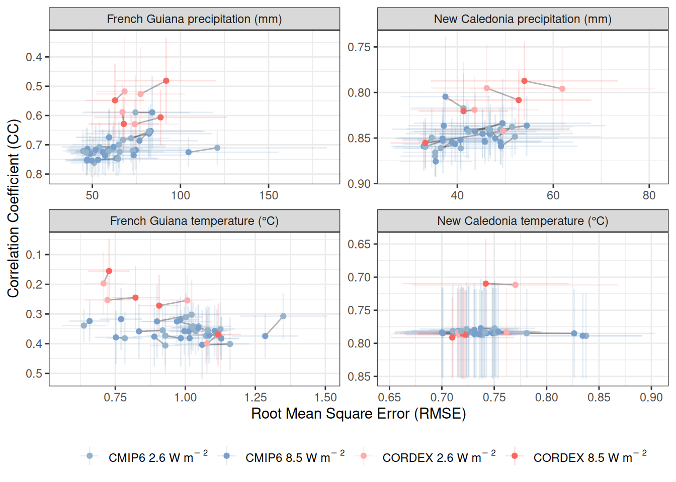
Fig S6. Evaluation of downscaled projections from global (CMIP6) and regional (CORDEX) climate models. Monthly precipitation and mean temperature from climate models were downscaled against CHELSA2 data for the period 1980-2005 for French Guiana and Ivory Coast. We evaluated downscaled projected monthly precipitation monthly mean temperature against punctual Meteo-France data for the period 2006-2019 with a minimum of 6 complete years. The x-axis represents the root mean square error (RMSE) and the y-axis the correlation coefficient (CC), such that the best evaluation is located in the lower left corner with a RMSEP of 0 and a CC of 1. Each point represents the mean evaluation across months of a single climate model for scenarios 2.6 or 8.5, with intervals around representing half the standard deviation across months. Blue dots represent CMIP6 global climate models with scenario 2.6 in light blue and 8.5 in dark blue, while red dots represent CORDEX regional climate models with scenario 2.6 in light red and 8.5 in dark red. Grey lines represent matching scenarios for a single model.

Code

t <- read_tsv("outputs/eval_meteofrance.tsv") %>%
  mutate(area = gsub("-", " ", area)) %>%
  filter(
    variable %in% c("tas", "pr"),
    type == "downscaled",
    metric %in% c("RMSE", "CC")
  ) %>%
  mutate(variable = recode(variable,
    "pr" = "precipitation",
    "tas" = "temperature"
  )) %>%
  mutate(base_eval = "Météo France") %>%
  group_by(area, origin, type, variable, base_eval, metric, model) %>%
  summarise(value = mean(value)) %>% # inter-months
  group_by(area, origin, type, variable, base_eval, metric) %>%
  summarise(sd = sd(value), mean = mean(value)) %>% # inter-model
  mutate(value = paste0(round(mean, 3), " (", round(sd, 3), ")")) %>%
  select(-sd, -mean) %>%
  pivot_wider(names_from = origin, values_from = value) %>%
  ungroup() %>%
  mutate(Evaluation = paste(base_eval, variable)) %>%
  rename(Country = area, Metric = metric) %>%
  select(Country, Evaluation, Metric, CMIP6, CORDEX) %>%
  arrange(Country, Evaluation, Metric)
write_tsv(t, "figures/ts02.tsv")
read_tsv("figures/ts02.tsv") %>%
  kable(caption = "Table S2. Mean evaluation of downscaled CMIP6 and CORDEX projections between 2006 and 2019 against météo France precipitation and temperature data in French Guiana and New Caledonia. Numbers indicate root mean square error (RMSE) or correlation coefficient (CC) with mean followed by standard deviation in parentheses. CMIP6 and CORDEX assessments are averaged across months, models and scenarios.") # nolint

Table S2. Mean evaluation of downscaled CMIP6 and CORDEX projections between 2006 and 2019 against météo France precipitation and temperature data in French Guiana and New Caledonia. Numbers indicate root mean square error (RMSE) or correlation coefficient (CC) with mean followed by standard deviation in parentheses. CMIP6 and CORDEX assessments are averaged across months, models and scenarios.

Country	Evaluation	Metric	CMIP6	CORDEX
French Guiana	Météo France precipitation	CC	0.709 (0.04)	0.566 (0.056)
French Guiana	Météo France precipitation	RMSE	64.928 (16.158)	74.762 (9.647)
French Guiana	Météo France temperature	CC	0.356 (0.026)	0.268 (0.086)
French Guiana	Météo France temperature	RMSE	0.992 (0.153)	0.886 (0.174)
New Caledonia	Météo France precipitation	CC	0.848 (0.013)	0.815 (0.025)
New Caledonia	Météo France precipitation	RMSE	42.539 (5.761)	47.826 (7.626)
New Caledonia	Météo France temperature	CC	0.784 (0.003)	0.767 (0.038)
New Caledonia	Météo France temperature	RMSE	0.74 (0.031)	0.732 (0.02)